Shortest paths with charging
This is a writeup on the most interesting interview problem I’ve seen, given to me by a startup in 2019 as a “3-hour takehome.” I never got to find out if they liked my solution, as I withdrew my candidacy shortly after submitting it!
Problem
Find the quickest route for an electric drone between any two stations in a charger network.
The drone has a fixed range and travels at constant speed.
# Maximum distance a fully charged drone can travel, in km
RANGE = 365
# Maximum drone speed, in km/hr
SPEED = 95
We have each charger’s latitude and longitude, as well as its chargeRate (in km of range added per hour of charging).
charger = pd.read_csv('charger_locations.csv', index_col=0)
charger.head()
| chargerID | latitude | longitude | chargeRate |
|---|---|---|---|
| 1228 | 42.842720 | -71.693882 | 93.099972 |
| 3522 | 33.862824 | -111.893035 | 185.081106 |
| 3874 | 40.931264 | -74.780646 | 147.505829 |
| 4114 | 41.712718 | -123.596716 | 160.018785 |
| 4031 | 45.719785 | -90.693155 | 124.010269 |
The drone is initially fully charged. It moves between chargers along great circle routes. It may stop at any number of chargers and charge for any amount of time at each, provided it does not run out of juice.
Solution
This is a graph problem reminiscent of the classic single-pair shortest paths problem (SPSP). The key difference in our case is the concept of recharging, which prevents us from simply assigning weights to each edge in the graph (say, for the travel time between two stations) and applying Dijkstra’s algorithm or $A^*$. Our first task will be to create a graph with charging stations as nodes and pairs of stations at most 365 km apart as edges and examining its structure.
We can compute the great circle distance between any two coordinate pairs using the haversine formula.
from math import radians, cos, sin, asin, sqrt

RADIUS_OF_EARTH = 6371

def great_circle_distance(lat1, lon1, lat2, lon2):
    lon1, lat1, lon2, lat2 = map(radians, [lon1, lat1, lon2, lat2])
    a = (sin((lat2 - lat1) / 2)**2
        + cos(lat1) * cos(lat2) * sin((lon2 - lon1) / 2)**2)
    return 2 * asin(sqrt(a)) * RADIUS_OF_EARTH
The number of chargers is small enough that we can precompute and store all ~90K pairwise great circle distances between chargers. (And we don’t even have to get clever with vectorization!)
import pandas as pd

dists = pd.DataFrame(0, index=charger.index, columns=charger.index)

for i in range(len(charger)):
    for j in range(i+1, len(charger)):
        d = great_circle_distance(
            charger.iloc[i]['latitude'], charger.iloc[i]['longitude'],
            charger.iloc[j]['latitude'], charger.iloc[j]['longitude']
        )
        dists.iloc[i, j] = d
        dists.iloc[j, i] = d

dists.iloc[:5, :5]
| chargerID | 1228 | 3522 | 3874 | 4114 | 4031 |
|---|---|---|---|---|---|
| 1228 | 0.000000 | 3607.368912 | 332.324867 | 4203.001200 | 1542.014089 |
| 3522 | 3607.368912 | 0.000000 | 3344.653973 | 1346.707558 | 2228.796521 |
| 3874 | 332.324867 | 3344.653973 | 0.000000 | 4021.603235 | 1389.878241 |
| 4114 | 4203.001200 | 1346.707558 | 4021.603235 | 0.000000 | 2662.309576 |
| 4031 | 1542.014089 | 2228.796521 | 1389.878241 | 2662.309576 | 0.000000 |
From our dists table we can compute travel times between each station pair, as well as a boolean matrix indicating which pairs of (distinct) stations the drone can travel between on a single charge.
travel_times = dists / SPEED
reachable = (dists <= RANGE) & (dists > 0)
Define a graph $G = (V, E)$ with adjacency matrix reachable, i.e. $V$ the set of charging stations and
Let’s see what $G$ looks like:
import networkx as nx
import matplotlib.pyplot as plt

G = nx.from_pandas_adjacency(reachable)

plt.figure(figsize=(20, 20))
node_positions = {
    cid: (charger.loc[cid, 'latitude'], charger.loc[cid, 'longitude'])
    for cid in charger.index
}
nx.draw(G, pos=node_positions, node_color=charger['chargeRate'])
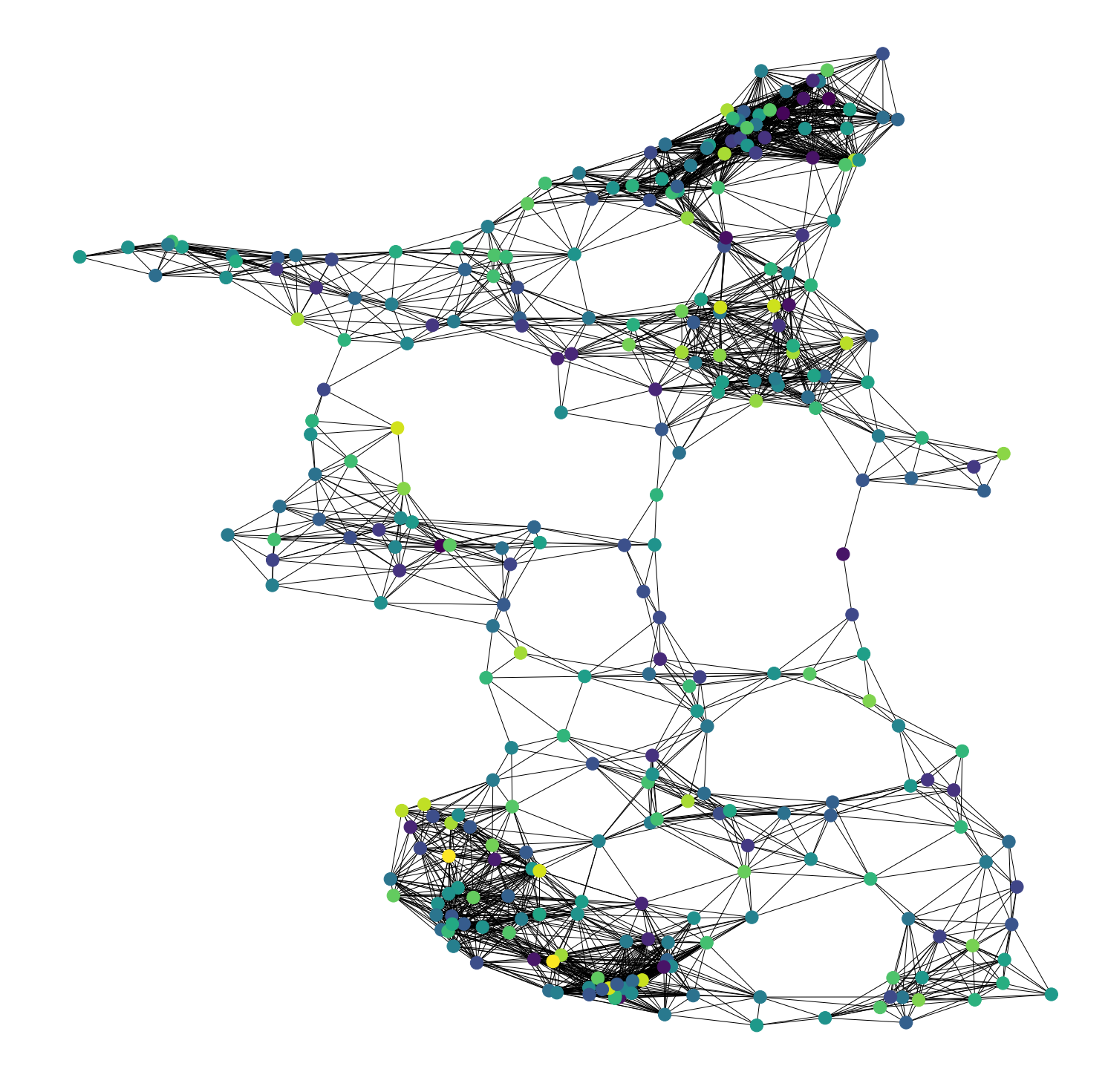
Since $G$ contains a single connected component and chargeRates are all positive, we know that there is a possible path for the drone between any two stations in the network. On average each station appears to have between 15 and 20 reachable neighbors.
Note that our problem reduces to SPSP in a few distinct limiting cases:
- in the limit as drone battery capacity reaches infinity;
- in the limit as charging rates at all stations approach infinity;
- in the limit as distances between stations approach 0.
In each of these cases the drone spends a negligible amount of time charging. In any of these regimes we expect a naive SPSP solution with charge times accounted for after the fact to approximate an exact solution to this problem reasonably well.
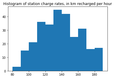
plt.hist(charger['chargeRate'], bins=np.arange(80, 200, 10))
plt.title('Histogram of station charge rates, in km recharged per hour')
plt.show()
import numpy as np

unique_dists = np.triu(dists.values * reachable.values).reshape(-1)
unique_dists = unique_dists[unique_dists > 0]
plt.hist(unique_dists, bins=np.arange(0, 400, 50))
plt.title('Histogram of distances between reachable pairs of charging stations')
plt.show()
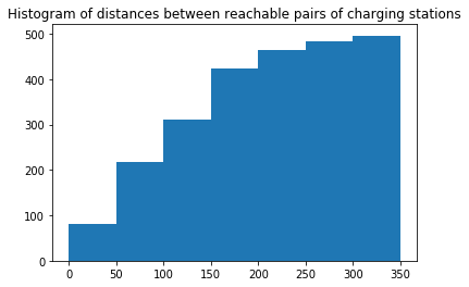
From these distributions it is clear that travel distances, charge rates, and drone range are all of the same order. Hence we don’t expect charge-agnostic SPSP to be a reasonable approximant for exact solutions.
Some commentary before we go on: I am aware of a variant of SPSP called the constrained shortest path problem (CSP) in which each edge is additionally associated with a quantity of resources consumed along the edge (say, fuel expenditure) and we must find the shortest path between two nodes subject to total resource expenditure not exceeding a given value. CSP is NP-hard, and on an intuitive level this problem seems at least as hard as CSP. So right off the bat I’m not too optimistic about finding a polynomial-time exact solution to this problem.
A subproblem I foresee being important to keep in mind is this:
Equator problem. Suppose the drone arrives at a station $s_1$ with no charge, must reach $s_3$, and the only possible path is $s_1 \to s_2 \to s_3$, all on the equator. Both legs of the journey take half battery and $s_1$ charges faster than $s_2$. A “greedy” algorithm would charge the drone only halfway at $s_1$, and then halfway again at $s_2$, never adding more charge than is necessary to complete the next leg. However, of course fully charging at $s_1$ and flying right over $s_2$ takes less time.
In my experience elegant solutions to graph problems often come from constructing some augmented graph $G’ = (V’, E’)$ from the base graph $G$ and applying a well-known algorithm (e.g. Dijkstra’s) to $G’$. Let’s see if we can do that here.
Recall that the reason we cannot assign time-denominated edge weights between reachable station pairs is because we do not know a priori how much time the drone should spend charging at the destination (cf. equator problem). But what if we let nodes in $G’$ correspond to state tuples $(v, \rho_v)$, where $\rho_v$ is the remaining range of the drone after charging at station $v$? Then the time between exiting $(u, \rho_u)$ and exiting $(v, \rho_v)$ is well-defined as
\[\text{dt}((u, \rho_u), (v, \rho_v)) = \text{travel_time}(u, v) + \frac{\rho_v - (\rho_u - \text{dist}(u, v))}{\text{charge_rate}(v)}.\]But the immediate issue is that the space of possible $\rho_v$ is infinite. How do we deal with this if we are to do computation on $G’$?
An immediate option is to discretize $\rho_v$ to $k+1$ levels such that $|V’| = (k+1)|V|$. That is, require $\rho_v \in \{ 0, R/k, 2R/k, \dots, R \}$, where $R$ is the drone’s range. We should draw an edge $((u, \rho_u), (v, \rho_v))$ in $G’$ only if the drone leaves $u$ with enough charge to make it to $v$, i.e. $\rho_u \geq d(u, v)$. I expect that in the limit as $k \to \infty$ the SPSP solution on $G’$ converges in some sense to an exact solution to our problem, though of course increasing $k$ comes at increased (quadratic) computational cost.
def cid_range_pairs(cid, k):
    return [(cid, i * RANGE / k) for i in range(k + 1)]

def build_modified_graph(G, k):
    Gp = nx.Graph()
    for cid in G.nodes:
        Gp.add_nodes_from(cid_range_pairs(cid, k))
    for (cid1, cid2) in G.edges:
        for (u, rho_u) in cid_range_pairs(cid1, k):
            for (v, rho_v) in cid_range_pairs(cid2, k):
                if rho_u < dists.loc[u, v]:
                    continue
                charge_time_at_v = (
                    (rho_v - rho_u + dists.loc[u, v])
                        / charger.loc[v, 'chargeRate']
                )
                if charge_time_at_v < 0: # Drone can't "de-charge"
                    continue
                Gp.add_edge(
                    (u, rho_u),
                    (v, rho_v),
                    dt=travel_times.loc[u, v] + charge_time_at_v
                )
    return Gp

Gp = build_modified_graph(G, 5)
We’ll now put everything together by wrapping the construction of $G’$ and Dijkstra’s algorithm into a function:
def shortest_path(G, k, start_cid, dest_cid):
    Gp = build_modified_graph(G, k)
    # Consider full range of final charge states at destination
    paths = []
    for _, final_charge in cid_range_pairs(dest_cid, k):
        try:
            paths.append(
                nx.dijkstra_path(
                    Gp,
                    source=(start_cid, RANGE),
                    target=(dest_cid, final_charge),
                    weight='dt'
                )
            )
        except:
            continue
    return paths

shortest_path(G, 5, 1228, 3522)[0]
[(1228, 365),
 (3047, 219.0),
 (840, 146.0),
 (3874, 219.0),
 (1572, 73.0),
 (936, 292.0),
 (473, 73.0),
 (2850, 365.0),
 (263, 219.0),
 (803, 365.0),
 (353, 73.0),
 (686, 292.0),
 (3733, 219.0),
 (401, 292.0),
 (4385, 146.0),
 (2645, 219.0),
 (1634, 73.0),
 (1015, 365.0),
 (148, 219.0),
 (2254, 292.0),
 (3522, 73.0)]
I decided to stop here. Right now shortest_path returns a list of optimal Dijkstra paths to the destination station at each possible final charge state. Because of our discretization of charge states we do not reach the destination with exactly 0 charge, and in fact we spend some time charging at the destination. I still have to modify it to choose the single optimal path and to include charge times at each station, but this is very straightforward. Given more time I’d like to carry out some simulations to see what effect varying $k$ has on the solution and/or try to prove convergence in the limiting case. Some other questions I’m interested in / initial ideas I didn’t implement:
- Suppose we apply charge-agnostic SPSP to $G$ and find shortest path $p_0$. We then remove the $v \in p_0$ with slowest
chargeRatefrom $G$ and run SPSP again to obtain $p_1$. We repeat this $m$ times and return $p^* = \arg \min_{j=0}^m \text{time}(p_j)$. Does $p^*$ approach an optimum as $m$ grows? - Can we solve this using dynamic programming? How can our DP solution avoid the pitfalls of the equator problem?
- In the real world this would be a stochastic optimization problem given that charging stations can go out of service or fill up, charging and battery burn rates can change, etc. How can we extend these ideas to the stochastic realm?